Mutating branching processes in deteriorating environments

One often encounters the problem of a branching process in a changing environment. Let's assume that the environment is changing such that birth rates behave as $$b = 1 + x - vt$$ while death rates are constant at $d=1$. This situation is a typical model of a lineages in an adapting population where $vt$ is the increasing mean fitness of the population. In order to survive, the lineage has to adapt and keep up with the increasing mean fitness. Let's assume a general mutation process with step site distribution $\mu(s)$ and a total mutation rate $\mu = \int ds \mu(s)$. One straightforward way to calculate the distribtion $p(n,t|x)$ of the number of descendants $n$ at time $t$ given the lineages started at fitness $x$ at time $t=0$ is via a first step equation. A first step equation (similar to a backward Fokker-Planck equation) varies with respect to the initial condition and expresses $p(n,t|x)$ as the whatever happens between $t=0$ and $t=\Delta t$ and $p(n,t-\Delta t | x - v\Delta t)$. Importantly, at $t=\Delta t$ the mean fitness of the population has increases by $v\Delta t$ and the growth rate of the focal lineage had decreased. The first step equation then reads $$p(n,t|x) = (1 - \Delta t (2+x+\mu))p(n,t-\Delta t|x-v\Delta t) + \Delta t \left[\delta(n=0) + (1+x)\sum_{n'=0}^n p(n', t|x)p(n-n', t|x) + \int ds \mu(s)(p(n,t|x-s) - p(n,t|x)) \right]$$ The first terms corresponds to nothing happening other than the clock advancing, while the terms in brackets correspond to death, division, and mutation. Rearranging and approximating the mutation terms by a Taylor series in small mutations, we have $$\dot{p}(n,t|x) + vp'(n,t|x) = -(2+x)p(n,t|x) + \delta(n=0) + (1+x)\sum_{n'=0}^n p(n', t|x)p(n-n', t|x) + \mu\langle s\rangle p'(n,t|x-s) + \frac{\mu \langle s^2\rangle}{2}p''(n,t|x)$$ To clean this up a little, let's define $\sigma^2 = v - \mu \langle s \rangle$ and $D = \frac{\mu \langle s^2 \rangle}{2}$. $$\dot{p}(n,t|x) = -(2+x)p(n,t|x) + \delta(n=0) + (1+x)\sum_{n'=0}^n p(n', t|x)p(n-n', t|x) - \sigma^2 p'(n,t|x-s) + Dp''(n,t|x)$$ Next, we consider the generating function $\hat{p}(\lambda, t|x) = \sum_{n=0}^\infty \lambda^n p(n,t|x)$. Multiplying the equation by $\lambda^n$ and summing over $n$ will factorize the convolution and turn the $\delta(n=0)$ into 1: $$\dot{\hat{p}}(\lambda,t|x) = -(2+x)\hat{p} + 1 + (1+x)\hat{p}^2 - \sigma^2 \hat{p}' + D\hat{p}''$$ This equation can be further simplified by substituting $\phi = 1 -\hat{p}$: $$\dot{\phi}(\lambda,t|x) = (2+x)(1-\phi) - 1 - (1+x)(1-\phi)^2 - \sigma^2 phi' + D\phi''$$ which after some rearrangment simplifies to $$\dot{\phi}(\lambda,t|x) = x\phi - \sigma^2 \phi' + D\phi'' - (1+x)\phi^2$$ The initial condition is $\phi(\lambda, t=0|x)= 1-\sum_n \lambda^n p(n,t=0|x)=1-\lambda$ when starting from one individual at fitness $x$.

The mean number of descendents

The mean $\langle n\rangle(t|x) = -\frac{d\phi}{d\lambda}(\lambda=1)$. We can therefore derive the following equation for the mean $$\dot{\langle n\rangle}(t|x) = x\langle n\rangle - \sigma^2 \langle n\rangle' + D\langle n\rangle'' - 2(1+x)\phi|_{\lambda=1} \langle n\rangle$$ where the last term is identical zero since $\phi==0$ if the initial condition is $\lambda=1$ (all terms in the evolution equation for $\phi$ vanish if $\phi=0$). This equation has the solution $$\langle n\rangle(t,x) = e^{xt - \frac{\sigma^2t^2}{2} + \frac{Dt^3}{3}}$$ The clone initally starts growing but the growth rate is gradually declining due to increasing mean fitness. During this time, the clone is diversifying and develops into a small traveling wave of its own. Selection on the increasing diversity attenuates the decline in growth rate. Only when the initial fitness is $>\frac{\sigma^4}{2D}$ is the growth rate always positive. This initial fitness corresponds to the positions of the most fit individuals in a traveling wave model.

Survival probability

The probability that there is at least one descendant at time $t$ is $$p_s = 1 - p(0,t|x) = 1 - \hat{p}(0,t|x) = \phi(0,x,t)$$ With initial condition $\lambda=0, \phi=1$, the solution for $\phi$ undergoes different characterisitic phases. At small times, $\phi$ is flat and none of the derivatives are important. Furthermore, typical fitness differentials are small ($|x|\ll 1$) such that the initial dominant balance is $\dot{\phi} = -\phi^2$ with solution $$\phi(t|x) = \frac{1}{1+t}$$ Hence the branching process is initially insensitive to growth rate differences and behaves like a critical branching process. Only after $t\sim 1/x\gg1$ is the selection term important. At large $x$, the dominant balance shifts to $x\phi = (1+x)\phi^2$ and therefore $\phi = x/(1+x$. This is the same result as you would find for a standard super-critical branching process: The lineage needs to escape initial stochastic loss, but once established grows fast enough to outrun the adapting population. This dominant balance will remain valid above $x_c = \frac{\sigma^4}{2D}$.

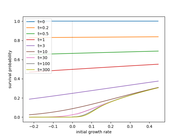
Below $x_c$, the increasing mean fitness strongly reduces the fixation probability. Ignoring the $\phi^2$ term, the remaining linear equation at steady state $$0 = x\phi - \sigma^2 \phi' + D\phi''$$ Has a solution in terms of Airy functions. The relevant solution goes to zero at large negative $x$ and crosses over to the linear

The script below solves for the survival probability at different times (via a very simple minded forward Euler solution of the differential equation).

import numpy as np
import matplotlib.pyplot as plt


def dphidt(phi,x,D,v):

    dphidx = np.zeros_like(phi)
    dphidx[1:-1] = (phi[2:] - phi[:-2])/(x[2:] - x[:-2])
    dphidx[0] = (phi[1] - phi[0])/(x[1] - x[0])
    dphidx[-1] = (phi[-1] - phi[-2])/(x[-1] - x[-2])

    dphidx2 = np.zeros_like(phi)
    dphidx2[1:-1] = 0.25*(phi[2:] - 2*phi[1:-1] + phi[:-2])/(x[2:] - x[:-2])**2

    return x*phi - v*dphidx + D*dphidx2 - (1+x)*phi**2


D = 0.0005
v = 0.002
dt = 0.01

tp = [0,.2,0.5,1,3,10,30,100,300]
x=np.linspace(-5*np.sqrt(v), 10*np.sqrt(v), 151)
phi = np.ones_like(x)
i=0
t=0

plt.figure()
while True:
    if t>=tp[i]:
        plt.plot(x, phi, label='t='+str(tp[i]))
        i+=1
        if (i==len(tp)):
            break
    phi+= dt*dphidt(phi, x, D, v)
    t+=dt

plt.legend(loc=2)
plt.plot([0,0], [0, 1], c='k', alpha=0.1)
plt.plot(x[x>0], (x/(1+x))[x>0], c='k', alpha=0.1)
plt.ylabel('survival probability')
plt.xlabel('initial growth rate')