How do things move around in a cell?
It is difficult to track single molecules. But it is reasonably straight forward to measure concentrations of many molecules. One convenient way to do so is by bleaching of fluorescent molecules with a strong laser. Say you labeled your molecule of interest with a small fluorescent dye that bleaches due to photo damage during strong illumination. If you now bleach the dye in some fraction of your field of view, you have set up a sharp gradient between fluorescent and non-fluorescent versions of your molecule. This method is called "Fluorescence Recovery After Photobleaching" or FRAP.
 Image by bioquant Heidelberg.
The recovery of the fluorescence signal is due to diffusion of intact GFP molecules into the space that was bleached.
Small object are constantly bounced around by thermal motions of surrounding molecules. This dynamics is called Brownian motion in honour of the botanist Robert Brown who noticed jittering of pollen grains under a microscope.
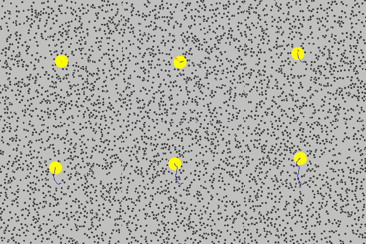 By Lookang Author of computer model: Francisco Esquembre, Fu-Kwun and lookang - Own work, CC BY-SA 3.0, Link
Despite (because) of the randomness of the process, the laws governing Brownian motion are simple and universal.
Discrete random walks
Consider a object at position \(x\) that at every time step moves 1 unit to the right with probability \(p\) and to the left with probability \(1-p\). Its displacement after \(n\) steps will be \(\Delta x = 2k-n\) where \(k\) is number of steps to the right. The distribution of displacements evidently follows a binomial distribution with
$$P(k,n) = \frac{n!}{k!(n-k)!}p^k(1-p)^{n-k}$$
The average displacement is simply given by
$$\langle \Delta x \rangle = 2\langle k \rangle - n = 2np \sum_k \frac{(n-1)!}{(k-1)!(n-k)!}p^{k-1}(1-p)^{n-k} - n = (2p-1)n$$
For a symmetric random walk with \(p=0.5\), the average displacement is zero as expected for random walks. This expression characterizes the average behavior, but the essence of Brownian motion lies in their randomness. To quantify the randomness in displacement, one typically looks at the mean squared deviation, the is the variance of the process.
$$\langle (\Delta x - \langle \Delta x\rangle)^2\rangle = \langle (2k-n - (2p-1)n)^2\rangle = 4\langle (k - p n)^2\rangle = 4\langle k^2 - p^2 n^2\rangle=4\langle k(k-1) + np - p^2 n^2\rangle$$
We have hence reduced the problem of calculating the variance to calculating the second moment. The very last step was merely a convenience transformation:
$$\langle k(k-1)\rangle= p^2 n(n-1)\sum_k \frac{(n-2)!}{(k-2)!(n-k)!}p^{k-2}(1-p)^{n-k} = p^2 n(n-1) $$
Plugging this back into the above, we get
$$\langle (\Delta x - \langle \Delta x\rangle)^2\rangle = (4\langle k(k-1) + np - p^2 n^2 = 4n(p-p^2) = 4np(1-p) $$.
The important observation is that the variance grows linearly with time, that is the number of steps \(n\). Since the variance is "distance squared", the typical displacement only grows with the square root of time. This is a universal property of diffusive processes: Due to the cancellation of random backwards and forward jitter, displacements don't grow linearly in time as they would in ballistic (directed) motion.
Master equations
Above, we have written down the probability distribution of the position of our random walker right away because we knew the answer from elementary combinatorics. We won't always be so lucky. So lets explore a more general way of looking at the problem. Consider the probability \(P(x,n)\) of observing our particle at position \(x\) at time \(n\). We can write down the following equation for the distribution at time \(n+1\):
$$P(x,n+1) = pP(x-1,n) + (1-p)P(x+1,n) $$
where the first term corresponds to hops towards the right, the second term to the left.
Very that the distribution from above \(P(x,n)\) solves this equation!
Diffusion in continuous time and space
Above we assumed that our particle is moved by a fixed amount at each time interval. That is of course not what actually happens. In reality, every object is bombarded by many molecules every nano-second and follows a continuous trajectory. Let make time continuous first and assume discrete left/right jumps happen with rate \(\nu\). \(P(x,t+\Delta t)\) the obeys
$$P(x,t+\Delta t) = (1-\nu\Delta t)P(x,t) + \frac{\nu\Delta t}{2} (P(x-1,t) + P(x+1,t)) $$
which can be rearranged into a differential equation
$$\frac{d P(x,t)}{dt} = \frac{\nu}{2} (P(x-1,t) - 2P(x,t) + P(x+1,t))$$
The combination of terms on the right is a discrete approximation of a second derivative that we'll come across again below.
Let's do away with the discrete steps and just assume that there is a certain function \(g(\delta x, \delta t)\) that describes the distribution of displacement \(\delta x\) after an infinitesimal time \(\delta t\). We can write
$$P(x,t+\Delta t) = \int d\delta x g(\delta x, \Delta t) P(x-\delta x, t) \approx \int d\delta x g(\delta x, \Delta t) \left[ P(x, t) - \delta x \frac{\partial P(x,t)}{\partial x} + \frac{\delta x^2}{2} \frac{\partial P(x,t)}{\partial x^2}\right]$$
where we assumed that \(\delta x\) remains small during the small time interval considered and expanded the distribution around \(x\). Rearranging yields
$$\frac{dP(x,t)}{dt} = - \frac{\langle\delta x\rangle_{\Delta t}}{\Delta t} \frac{\partial P(x,t)}{\partial x} + \frac{\langle \delta x^2\rangle_{\Delta t}}{2\Delta t}\frac{\partial P(x,t)}{\partial x^2}$$.
The coefficient \(v=\frac{\langle\delta x\rangle_{\Delta t}}{\Delta t}\) has the interpretation of a velocity: average displacement within time \(\Delta t\) divided by that time. The other coefficient has units \([displacement^2]/[time]\). We have seen above that mean squared displacement scales linearly in time in a simple discrete model. This holds more generally and we can define a time independent diffusion coefficient:
$$ \lim_{\Delta t \to 0} \frac{\langle \delta x^2\rangle_{\Delta t}}{2\Delta t} = D $$
The diffusion equation then takes the form
$$\frac{\partial P(x,t)}{\partial t} = - v\frac{\partial P(x,t)}{\partial x} + D\frac{\partial P(x,t)}{\partial x^2}$$.
Green's function of the diffusion equation
Depending on the initial and boundary conditions, the difusion equation admits different solutions. On important situation is the diffusion of particles that are initially localized at a point \(x=0\) and spread via diffusion.
$$ P(x,t) = \frac{1}{\sqrt{4\pi Dt}}e^{-\frac{(x-vt)^2}{4Dt}} $$
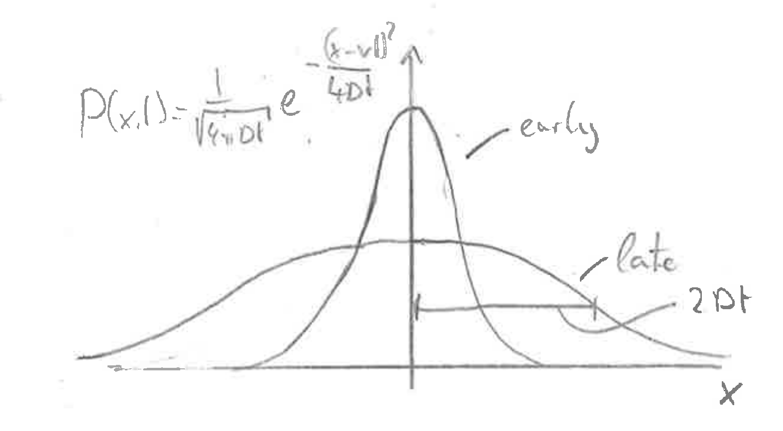
Verify that this is a solution!
Fluxes and boundary conditions
Whenever the distribution \(P(x,t)\) is inhomogenous, there is a net flux of particles. This is most readily seen by rewriting the diffusion equation as
$$ \frac{\partial P(x,t)}{\partial t} = -\frac{\partial}{\partial x}\left[ v P(x,t) - D\frac{\partial P(x,t)}{\partial x} \right] = - \frac{\partial}{\partial t} j(x,t) $$
where \(j(x,t)\) is the flux of particles. The parts of the flux have an intuitive interpretation: the term \(vP(x,t)\) describes how the density \(P(x,t)\) is moved by the advection velocity \(v\). The term \(D\frac{\partial P(x,t)}{\partial x}\) is the result of random diffusion: Whenever \(P(x,t)\) is falling, more particles remove from left to right than vice versa, resulting in a net flux towards the low density region. The expression for the flux is also known and Fick's law.
Fluxes are critical when we consider diffusion in a domain whose boundaries restrict fluxes. The most common boundary conditions are (i) no-flux boundaries (for example impermeable membranes), (ii) absorbing boundary conditions (for example a sticky surface), or (iii) constant flux boundary conditions where particles are injected at constant rate (for example a fly embryo with localized translation at one end of the embryo).
No flux boundary conditions
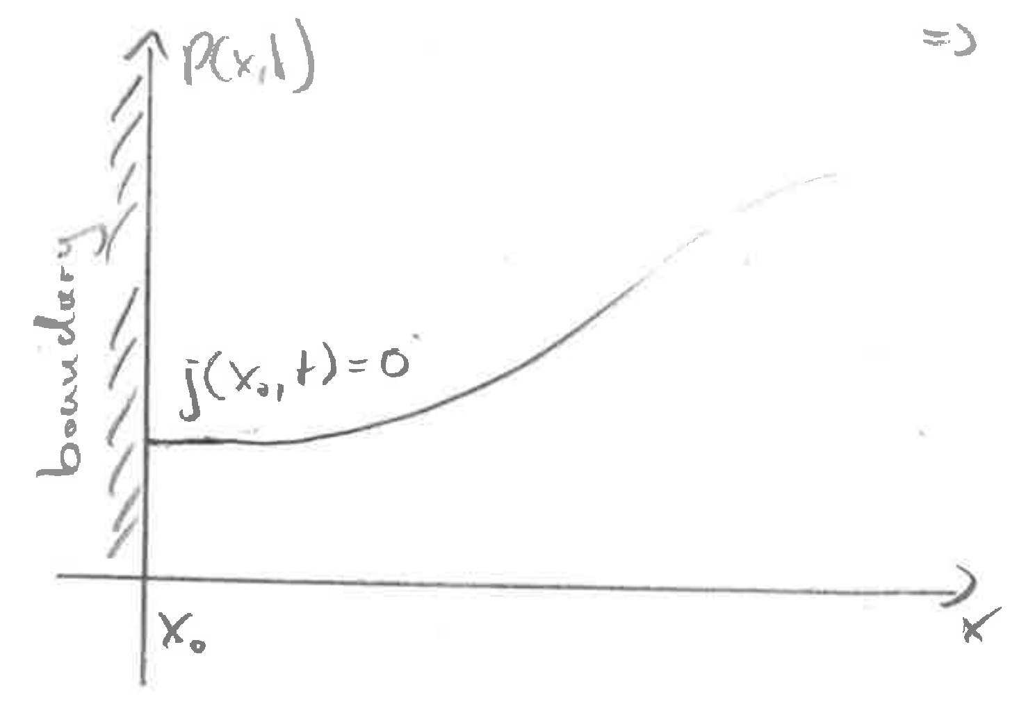 At the boundary, the flux \(j(x,t)\) has to vanish. This is achieved if \(DP'(x,t) = vP\) (note that there is a \(P\) missing in the graph). In the particular care of \(v=0\), this corresponds to zero slope.
Absorbing boundary conditions
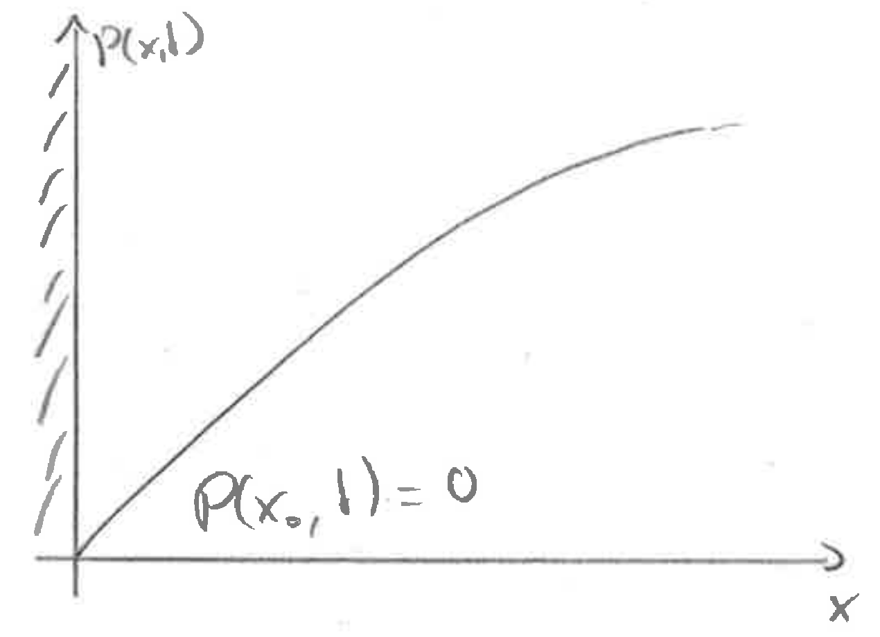 At an absorbing boundary, the density at the boundary has to equal zero (unless \(D\to 0\) at the boundary). The probability flux at the boundary is the rate of absorbtion.
The method of mirror sources
The Gaussian solution above extends to infinity.
In a bounded domain, we need a different solution!
One common strategy is to use the method of mirror sources. What this does is best appreciated in a picture:
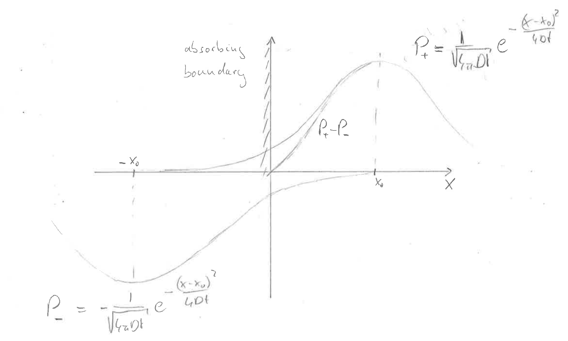 Consider a source at position \(x_0\) and an absorbing boundary at \(x=0\).
If we place a negative source at position \(x=-x_0\) and add those two contributions, the sum will go through zero at \(x=0\) as required.
This superposition of different solutions works because the diffusion equation is a linear equation.
$$P(x,t) = \frac{1}{\sqrt{4\pi Dt}}\left[e^{-\frac{(x-x_0)^2}{4Dt}} - e^{-\frac{(x+x_0)^2}{4Dt}}\right]$$
Calculate (evaluate) the rate at which probability is lost. What is the \(\int_0^\infty dx P(x,t)\)?
The same trick can be used for reflecting boundary conditions: The two contributions from \(x=x_0\) and \(x=-x_0\) need to be added rather than subtracted.
$$P(x,t) = \frac{1}{\sqrt{4\pi Dt}}\left[e^{-\frac{(x-x_0)^2}{4Dt}} + e^{-\frac{(x+x_0)^2}{4Dt}}\right]$$
Does this also work for \(v\neq 0\)?
Estimating diffusion coefficiencts from FRAP experiments
Before we start with sophisticated calculations it is useful to develop some intuition for the problem
- we want to estimate \(D\) with units \(length^2/time\)
- somehow, a length scale and a time scale need to be involved
- the length scale available is the size of the bleached window \(w\)
- a plausible time scale would be the time to 50% recovery in the middle \(t_{1/2}\)
Hence we would expect that the diffusion coefficient is roughly \(D\sim w^2/4t_{1/2}\).
Let's see how this simple reasoning compares to a more careful calculation. To makes things simpler, assume that we have bleach everything to the right of \(x=0\) such that our initial condition reads
$$ P(x,0) = \cases{ c & x<0 \cr 0 & x>0 } $$
Since we don't have any boundary conditions in our simplified set-up, we can express the solution as a superposition of many initial point sources distributed along the axis for \(x<0\).
$$P(x,t) = c \sum_{i} \frac{dx}{\sqrt{4\pi Dt}}e^{-\frac{(x+i dx)^2}{4Dt}}$$
This is a spiky solution with spacing \(dx\), but we can take the continuum limit and send \(dx\) toward zero. In this case we get:
$$P(x,t) = \frac{c}{\sqrt{4\pi Dt}} \int_{-\infty}^0 dx_0 e^{-\frac{(x - x_0 )^2}{4Dt}} = \frac{c}{\sqrt{4\pi Dt}} \int_{-\infty}^{x} dx_0 e^{-\frac{x_0^2}{4Dt}} = \frac{c}{2}\left[1 - \mathrm{erf}(x/\sqrt{4dt})\right]$$
This distribution is pathological at \(t=0\) because of an infinitely steep jump at \(x=0\) but for any \(t>0\) is fine.
In this example without any boundary conditions, the concentration will eventually settle at a uniform value if \(c/2\). Hence we might want to ask when the concentration at \(x=d>0\) has reached \(c/4\).
$$P(d,t_{1/2}) = \frac{c}{2}[1 - \mathrm{erf}(d/\sqrt{4Dt_{1/2}})] = \frac{c}{4}$$
which requires \(\mathrm{erf}(d/\sqrt{4Dt_{1/2}}) = 1/2\) and we get
$$D \approx 1.1\frac{d^2}{t_{1/2}}$$
We see that our simple scaling argument got us pretty close to the correct answer. The prefactor will differ for different geometries and initial conditions.
Typical diffusion coefficients
- GFP in eukaryotic cells: \(\sim 25 \mu m^2/s\)
- GFP in prokaryotic cells: \(\sim 10 \mu m^2/s\)
- mRNA (actin in mouse): \(\sim 0.2 \mu m^2/s\)
- \(\mathrm{H_2O}\) molecule in \(\mathrm{H_2O}\): \(\sim 2000 \mu m^2/s\)
- \(\mathrm{H^+}\) molecule in \(\mathrm{H_2O}\): \(\sim 7000 \mu m^2/s\)
→ protein: \(\sim 10\mu m^2/s\), small molecule: \(\sim 1000 \mu m^2/s\), big polymer: \(\sim 0.2 \mu m^2/s\).
How long does it take for a protein to diffuse a distance \(x\)?
The typical distance scale after a time \(t\) is
$$ \Delta x = \sqrt{2Dt} \quad \Rightarrow \quad t = \frac{\Delta x^2}{2D}$$
- \(\Delta x = 1\mu m\): \(t = 0.05s\) [across a bacterium]
- \(\Delta x = 10\mu m\): \(t = 5s\) [across a eukaryotic cell]
- \(\Delta x = 1000\mu m\): \(t = 5000s=83m\)
- \(\Delta x = 1m\): \(t = 5\times 10^9s=160y\) [along a peripheral axon]
→ diffusion is fast on short distances, but completely inadequate on long distances.