Analysing SARS-COV-2 data
This is the last part of the Qlife Nextstrain workshop. One can either try things with their own data or choose to focus on SARS-COV-2. This document provides some guidelines to the SARS-COV-2 analysis.
Questions
These are some suggestions concerning the questions you should try to answer using Nextstrain. Feel free to focus on other questions if you have something specific in mind. - How many clades is there in your data ? What do they correspond to ? - How fast does SARS-COV-2 evolve overall ? - Is the root of the tree correctly inferred ? - Where are most of the mutations happening ? What does this gene correspond to ? - What are some of the mutations characterizing the different variants ?
Downloading sequence dataset
Use online resources to create a SARS-COV-2 sequence dataset of around 10 000 sequences. In our case we will be using NCBI website to get those sequences: https://www.ncbi.nlm.nih.gov/sars-cov-2/.
Click there to access the sequence download page
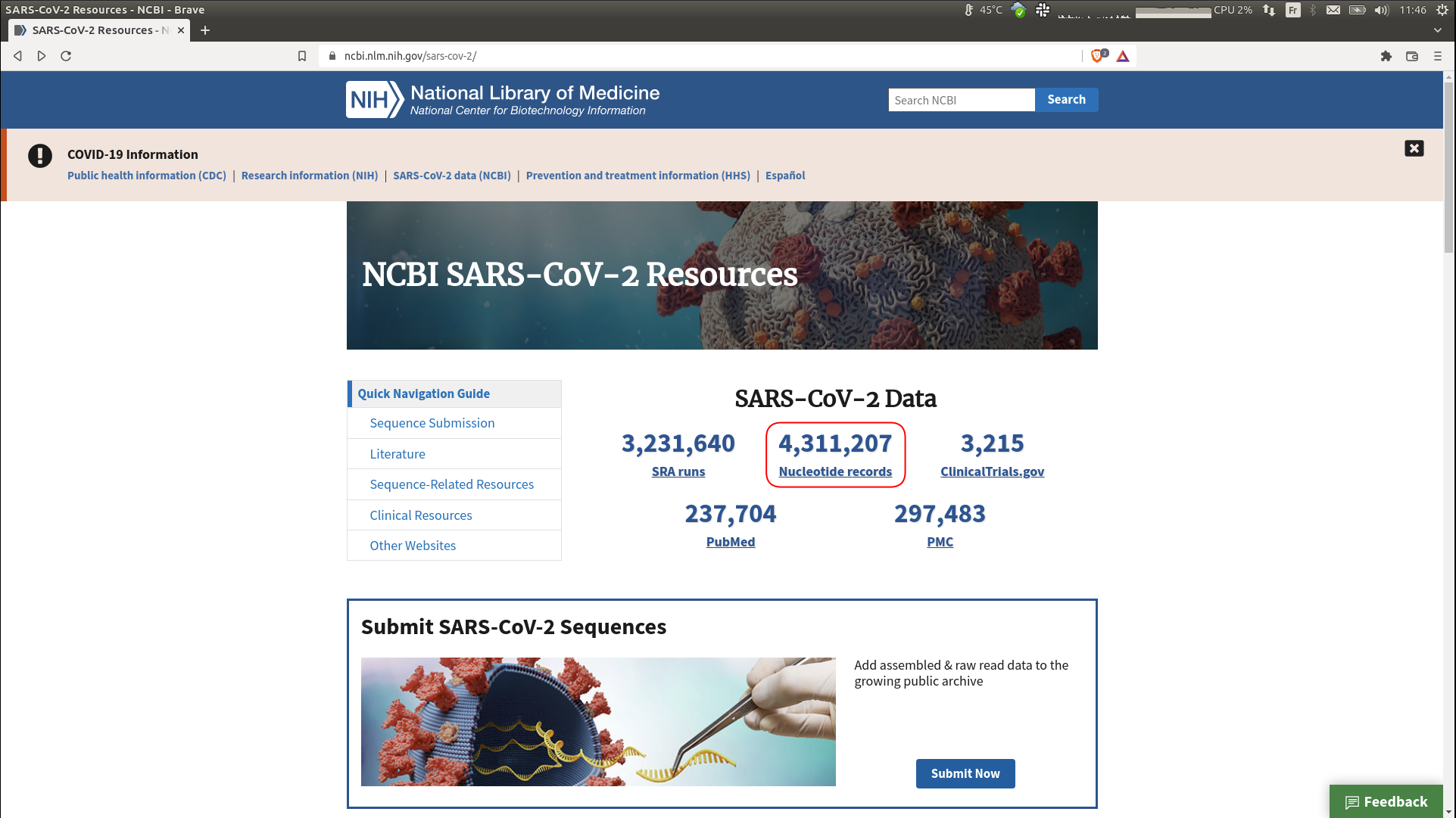
You will arrive there
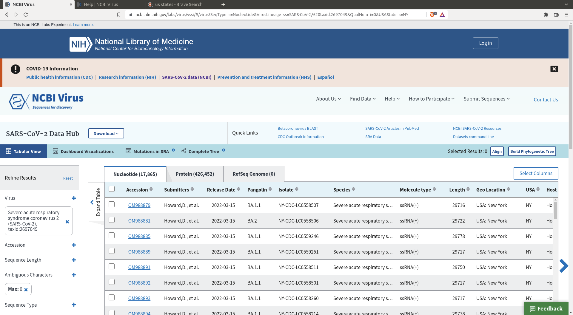
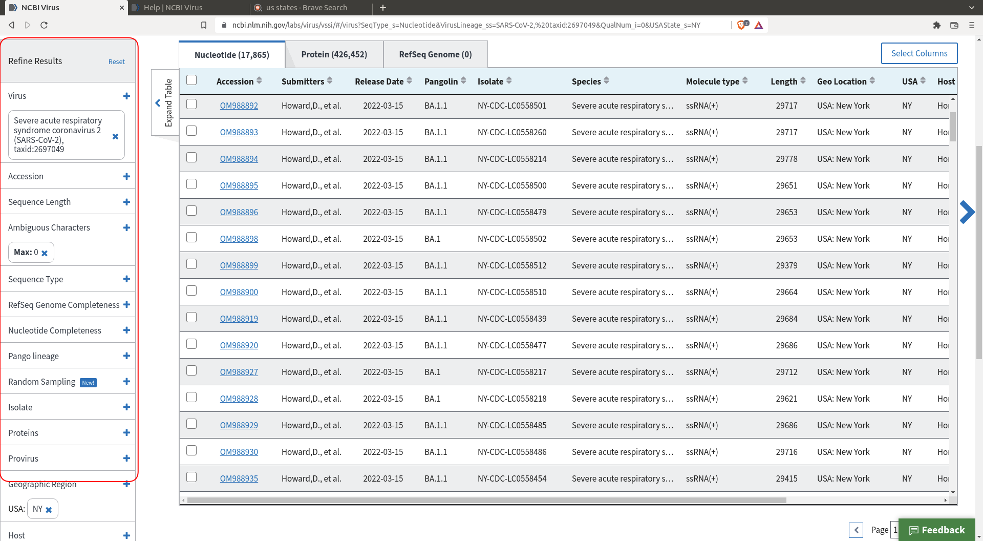
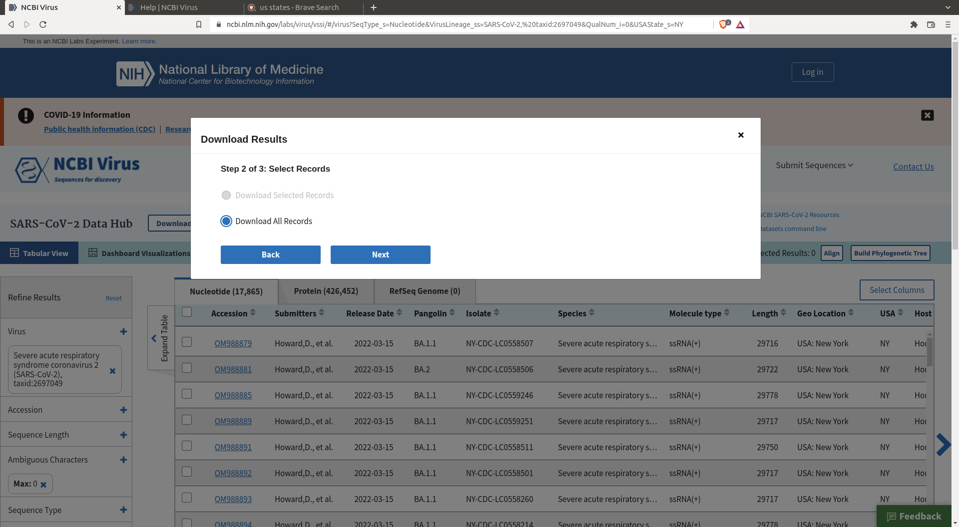
Do a selection of the sequences you want. I my case I selected sequences coming from New York that have no ambiguous character (there are enough sequences so we might as well remove the messy ones).
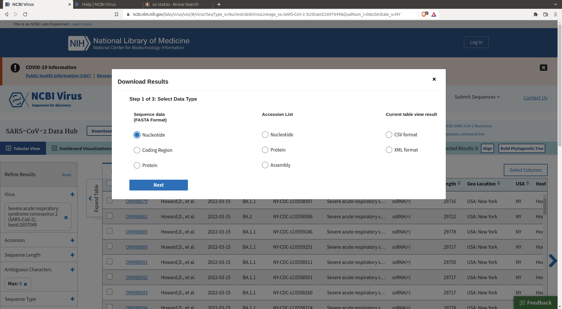
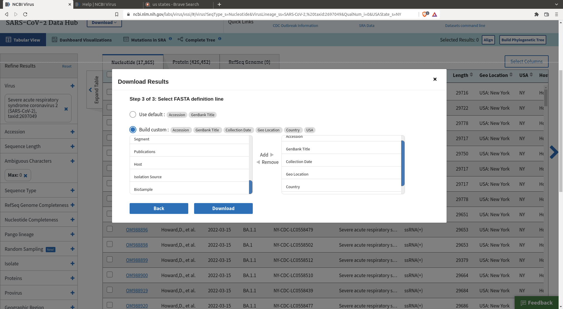
Then click download and define the header you want for your sequences
One also needs a reference sequence for the future alignment : https://www.ncbi.nlm.nih.gov/nuccore/MN908947.3/
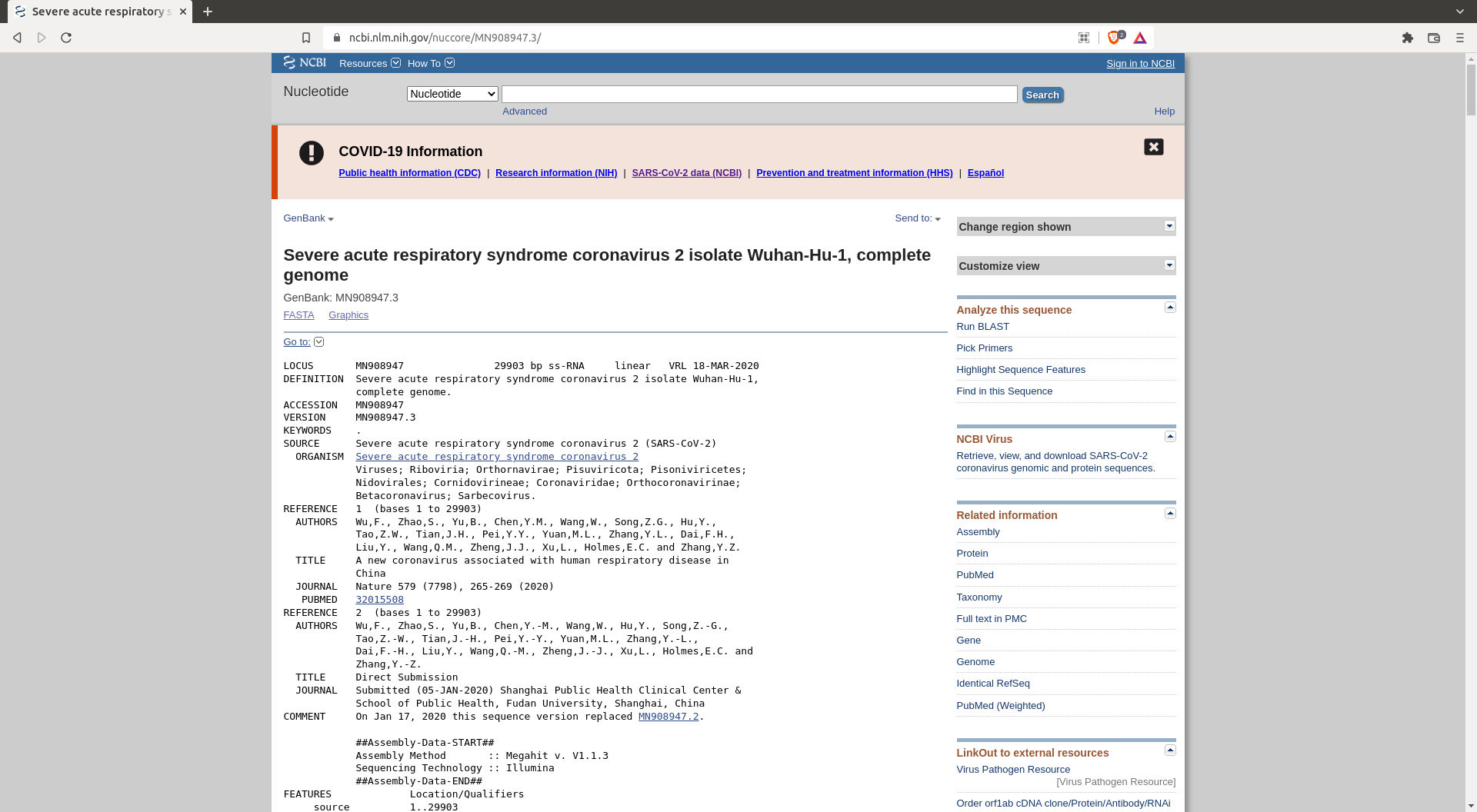 Take this sequence and save it as
 reference.gb in your data folder.
Curating the dataset
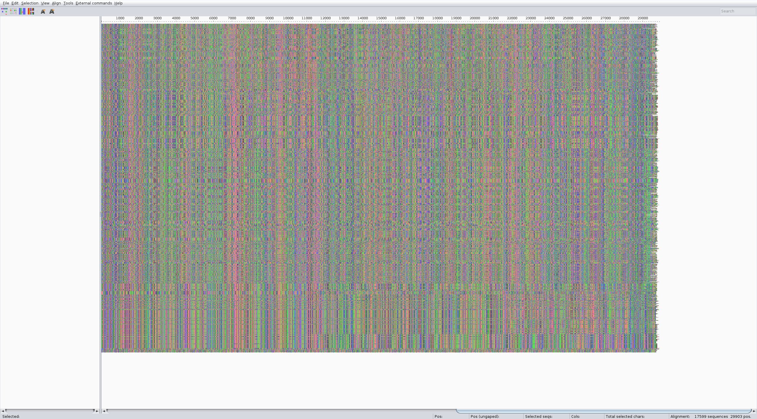
Look at what you get on Aliview or similar. It's around 500mb
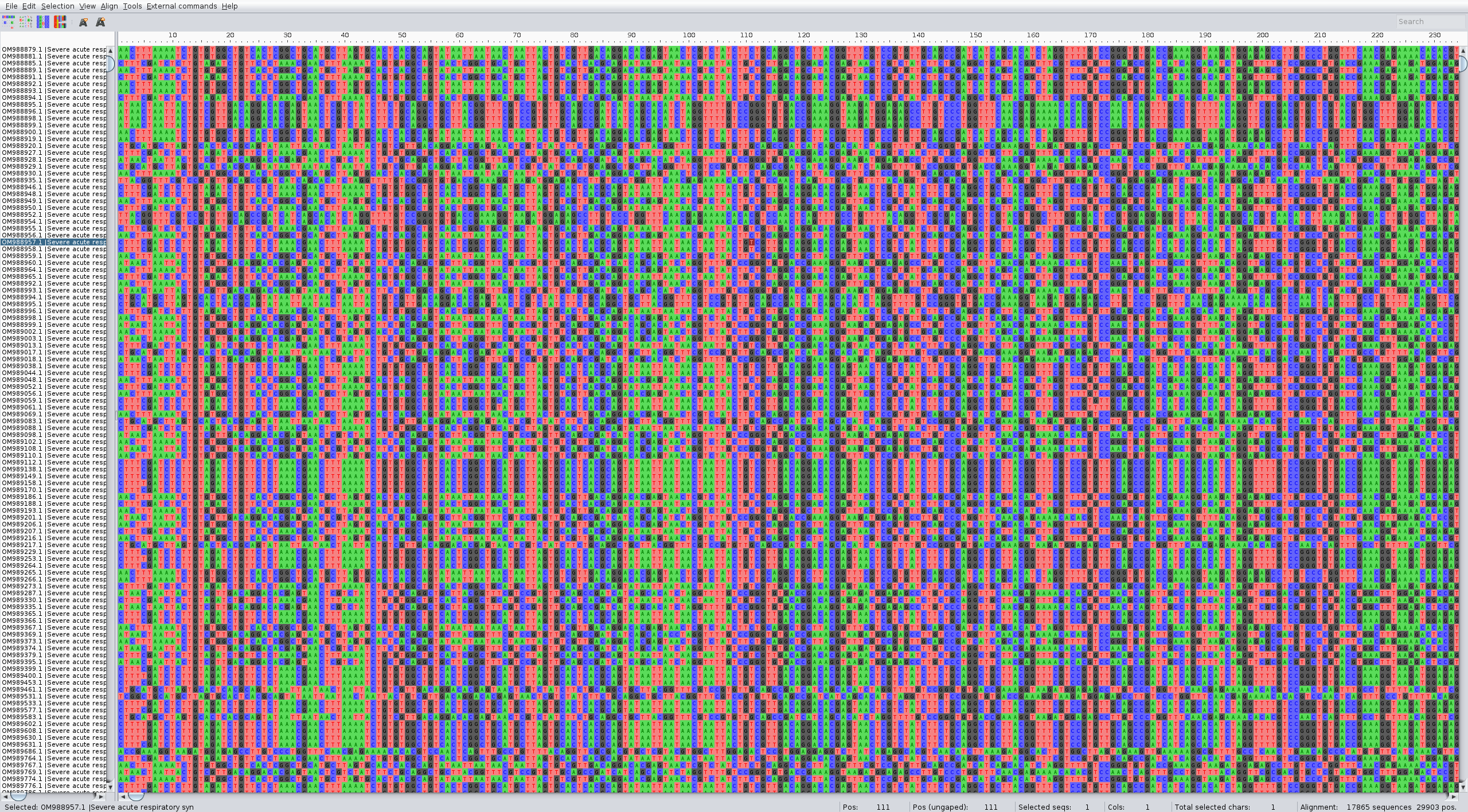
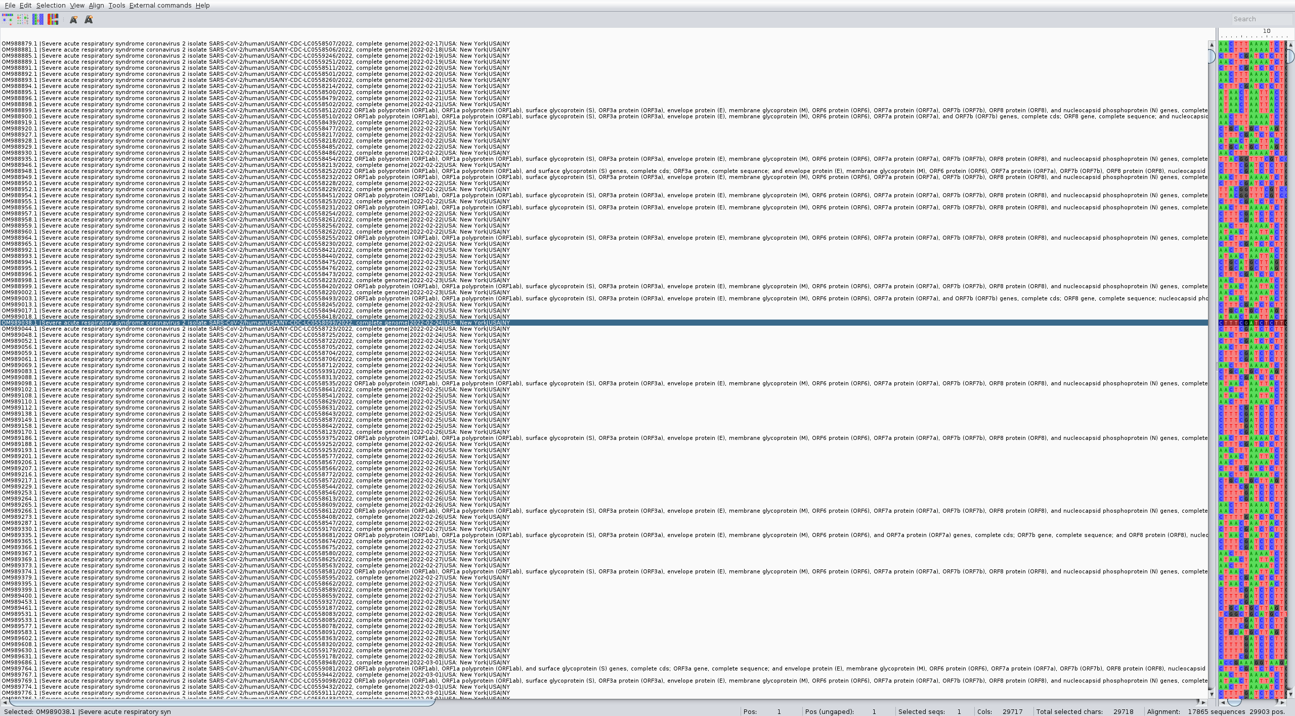
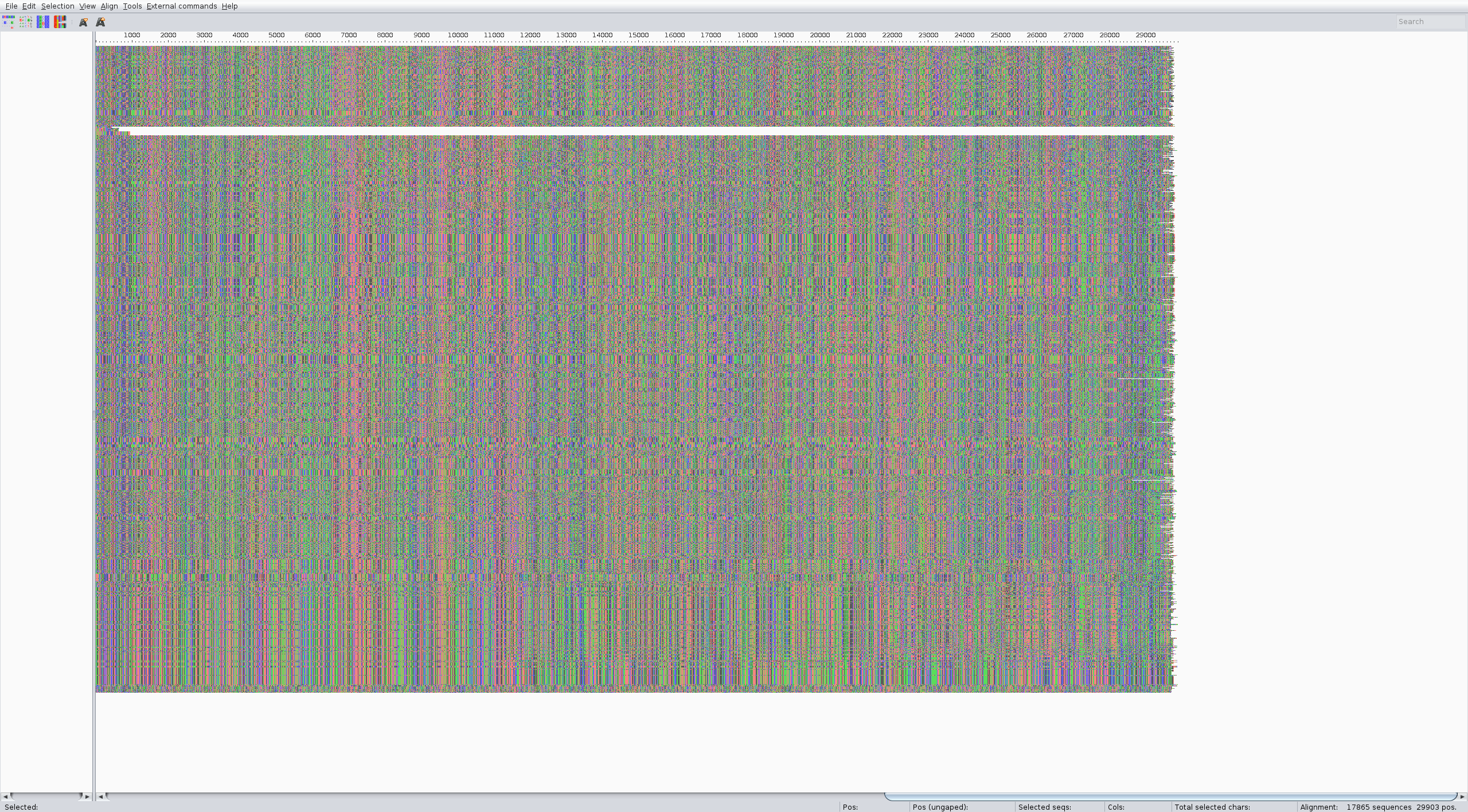
As you can see the names are not good, and some sequences seem to be not complete
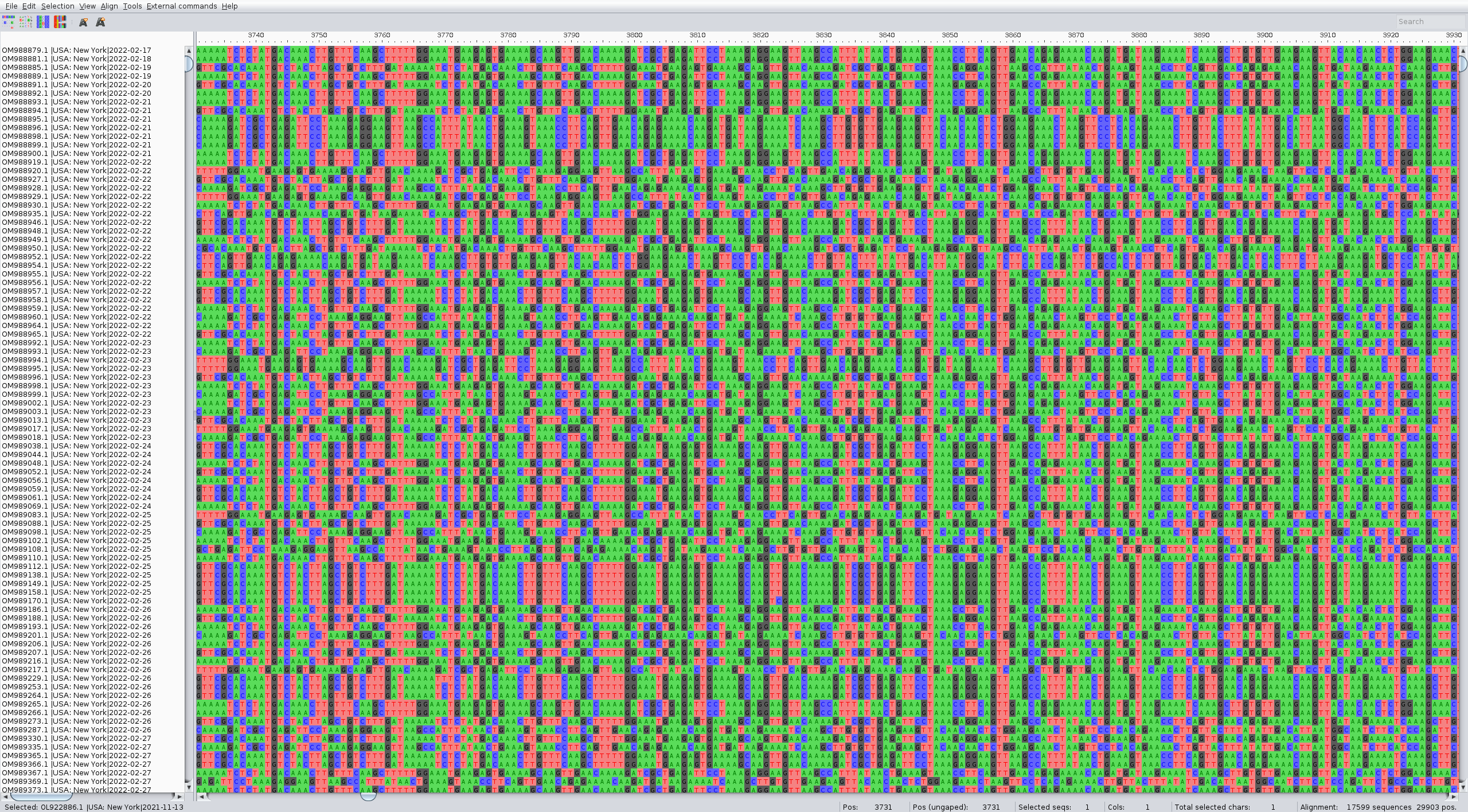
We could curate this data manually or with a script, but we can also do this by being a bit more restrictive when download the dataset. Go back to the download page and additionally select for sequence length. Then redefine the header in a more useful way
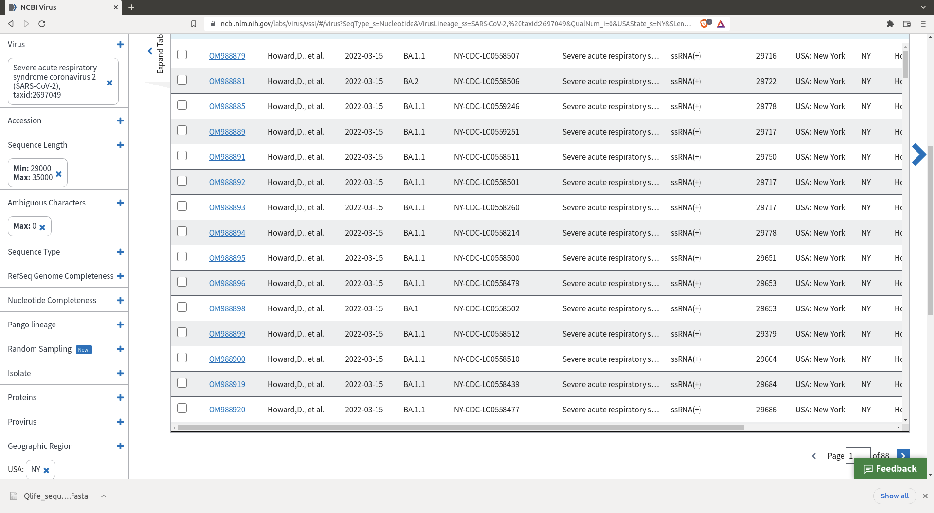
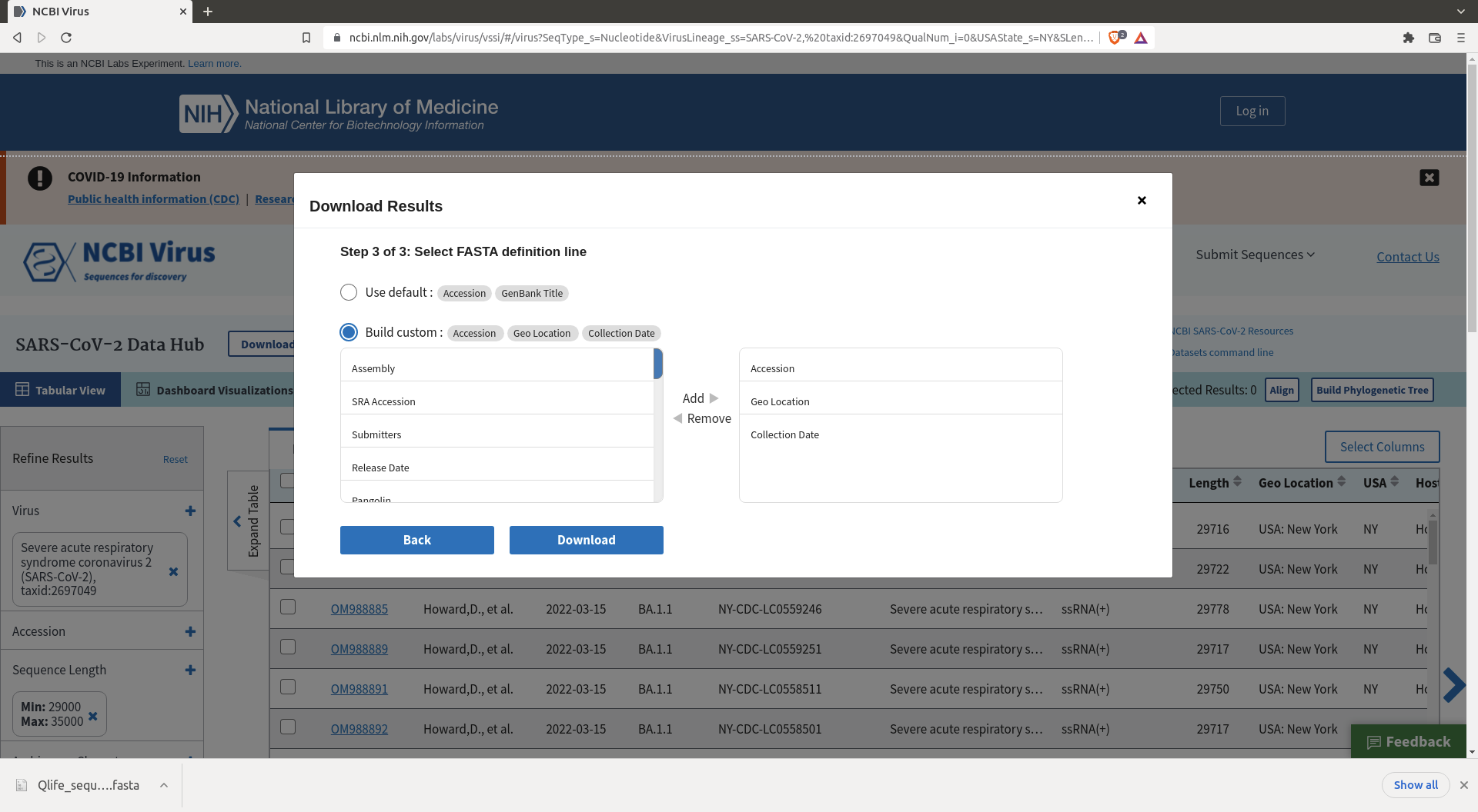
What you get now is better, only full sequences and with easier names
Building the pipeline
The steps are very similar to the zika tutorial, except that we must create the metadata file from the sequence names and change a bit the parameters in the filter part to correctly subsample the dataset. You need this subsampling step otherwise it the following steps will take a long time to run (too many sequences).
We suggest putting the raw data and everything you want to keep in a folder called data. The files that you want to clean from one analysis to the next will be in another folders that will be removed via a snakemake clean rule.
Now it is time to create the snakemake pipeline. You can inspire yourself from the zika tutorial as it will be very similar.
First define the input files you are going to use:
INPUT_FASTA = "data/Qlife_sequences.fasta",
REFERENCE = "data/reference.gb",
DROPPED = "data/dropped.txt"
AUSPICE_CONFIG = "auspice_config.json"
You need to create the dropped.txt file even if it stays empty.
Also define the cleaning rule:
rule clean:
    message: "Removing directories: {params}"
    params:
        "results",
        "visualisation"
    shell:
        "rm -rfv {params}"
Metadata
The metadata concerning our sequence si contained in their headers. To create the metadata from these headers one can use the augur parse command.
A snakemake rule can be created for this, for ex:
rule metadata:
    message:
        """
        Creating the metadata file from raw sequences {input.sequences}
        """
    input:
        sequences = INPUT_FASTA
    output:
        metadata = "data/metadata.tsv",
        sequences = "data/sequences.fasta"
    params:
        fields= "accession country date"
    shell:
        """
        augur parse \
            --sequences {input.sequences} \
            --output-sequences {output.sequences} \
            --output-metadata {output.metadata} \
            --fields {params.fields}
        """
Checking the metadata we see the "country" field is not always the same.
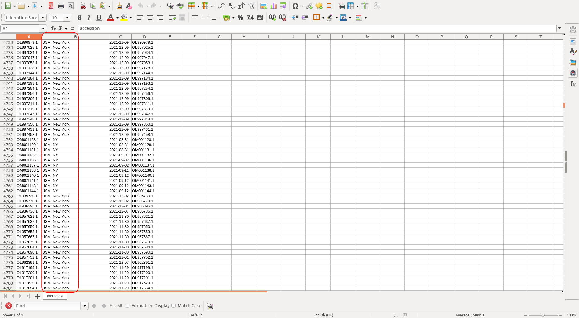
This needs to be fixed otherwise the subsampling part will not work correctly. One can use something like libreoffice calc to fix it manually, or create a small script (that you could include in a rule) to do so.
Subsampling
One needs to perform subsampling of the raw data to run the analysis in a reasonable amount of time. This can be done using the augur index command followed by the augur filter command. We suggest working with a small dataset of ~100 sequences while building the pipeline, then ~500-1000 sequences once it works.
Example for these two rules:
rule index_sequences:
    message:
        """
        Creating an index of sequence composition from {input.sequences}.
        """
    input:
        sequences = rules.metadata.output.sequences,
        metadata = rules.metadata.output.metadata
    output:
        sequence_index = "data/sequence_index.tsv"
    shell:
        """
        augur index \
            --sequences {input.sequences} \
            --output {output.sequence_index}
        """

rule filter:
    message:
        """
        Filtering to
          - {params.max_sequences} sequence(s) in total
          - from {params.min_date} onwards
          - excluding strains in {input.exclude}
        """
    input:
        sequences = rules.metadata.output.sequences,
        sequence_index = rules.index_sequences.output.sequence_index,
        metadata = rules.metadata.output.metadata,
        exclude = DROPPED
    output:
        sequences = "results/filtered.fasta",
        metadata = "results/filtered_metadata.tsv"
    params:
        group_by = "country year month",
        max_sequences = 100,
        min_date = 2010,

    shell:
        """
        augur filter \
            --sequences {input.sequences} \
            --sequence-index {input.sequence_index} \
            --metadata {input.metadata} \
            --output {output.sequences} \
            --output-metadata {output.metadata}\
            --group-by {params.group_by} \
            --subsample-max-sequences {params.max_sequences} \
            --min-date {params.min_date} \
            --exclude {input.exclude}
        """
Alignment
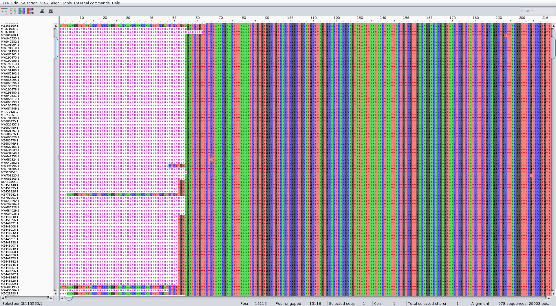
The alignment can be performed with the augur align command like in the zika tutorial. We suggest running it on several threads to speed up the process (4 is usually a good choice). It usually takes a couple of minutes. Inspect the result of the alignment (for ex. with Aliview) for quality control.
The rule should look like:
rule align:
    message:
        """
        Aligning sequences frpm {input.sequences} to {input.reference}
        """
    input:
        sequences = rules.filter.output.sequences,
        reference = REFERENCE
    output:
        alignment = "results/aligned.fasta"
    params:
        nthreads = 4
    shell:
        """
        augur align \
            --sequences {input.sequences} \
            --reference-sequence {input.reference} \
            --output {output.alignment} \
            --fill-gaps \
            --nthreads {params.nthreads}
        """
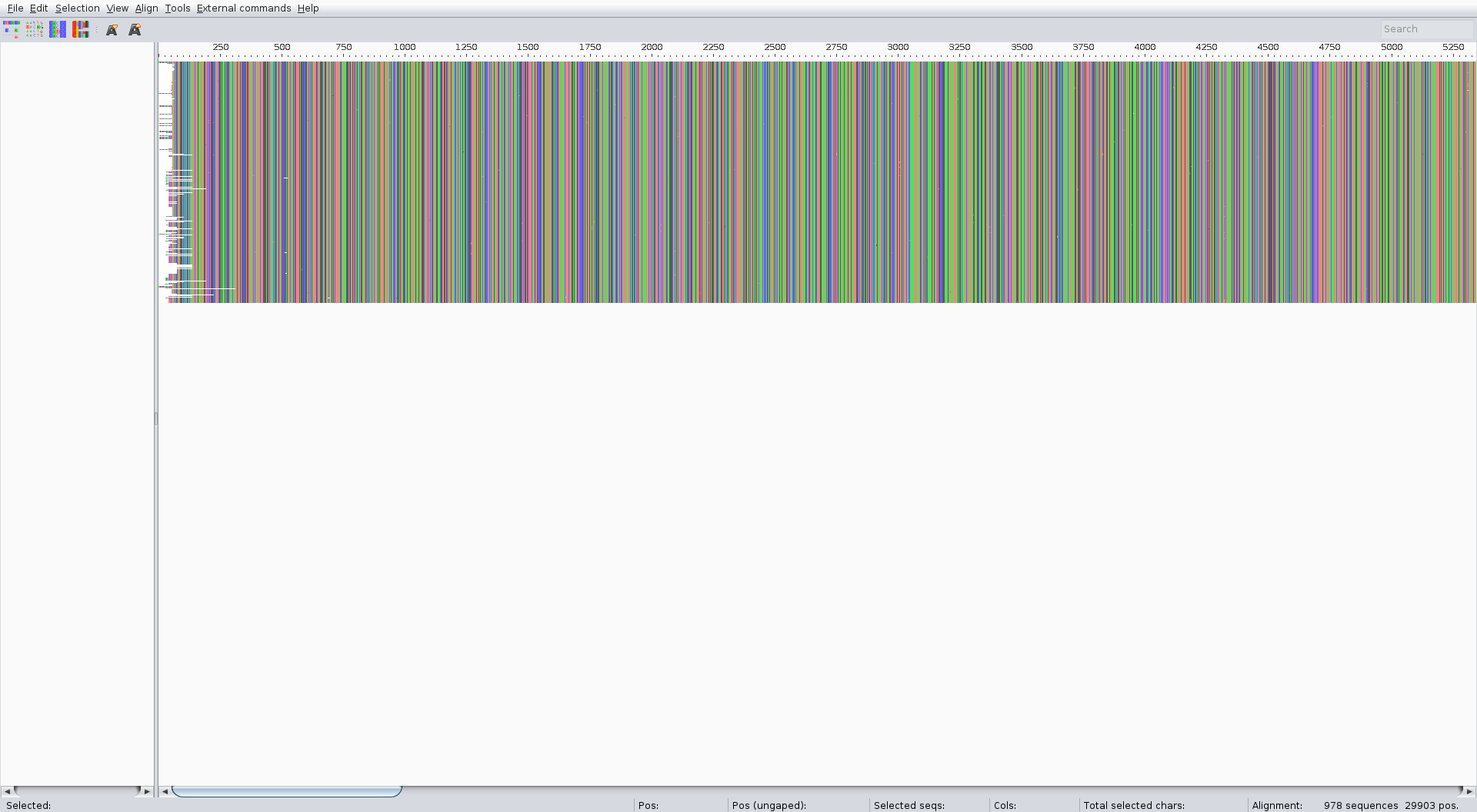
The alignment should look something like:
Tree
The phylogenetic tree is computed from the alignment with the augur tree command like in the zika tutorial. Once again we suggest running it on 4 threads. Inspect the tree once it's done. It can be done easily using the online version of Auspice: https://auspice.us/.
The rule should look like:
rule tree:
    message: "Building tree from {input.alignment}"
    input:
        alignment = rules.align.output.alignment
    output:
        tree = "results/tree_raw.nwk"
    params:
        nthreads = 4
    shell:
        """
        augur tree \
            --alignment {input.alignment} \
            --output {output.tree} \
            --nthreads {params.nthreads}
        """
Tree making should be fast (~1min)
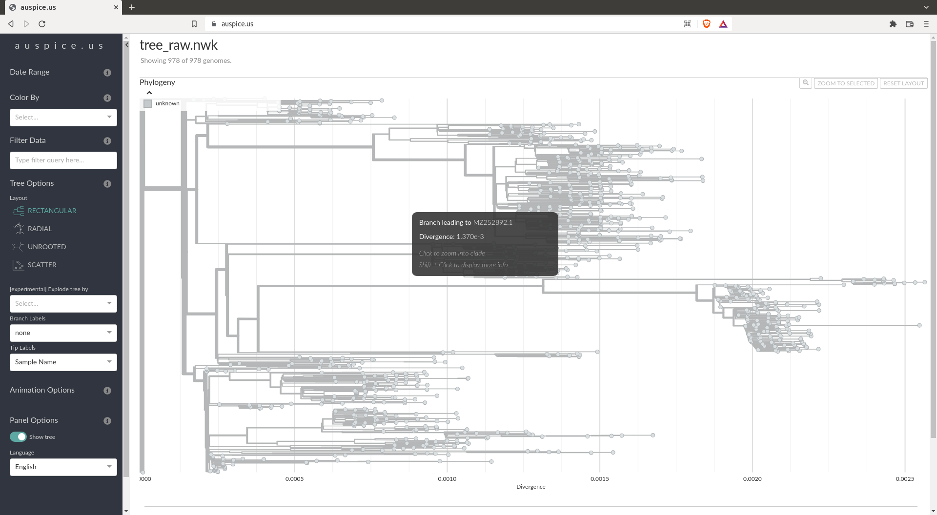
The tree should look like:
Tree refining
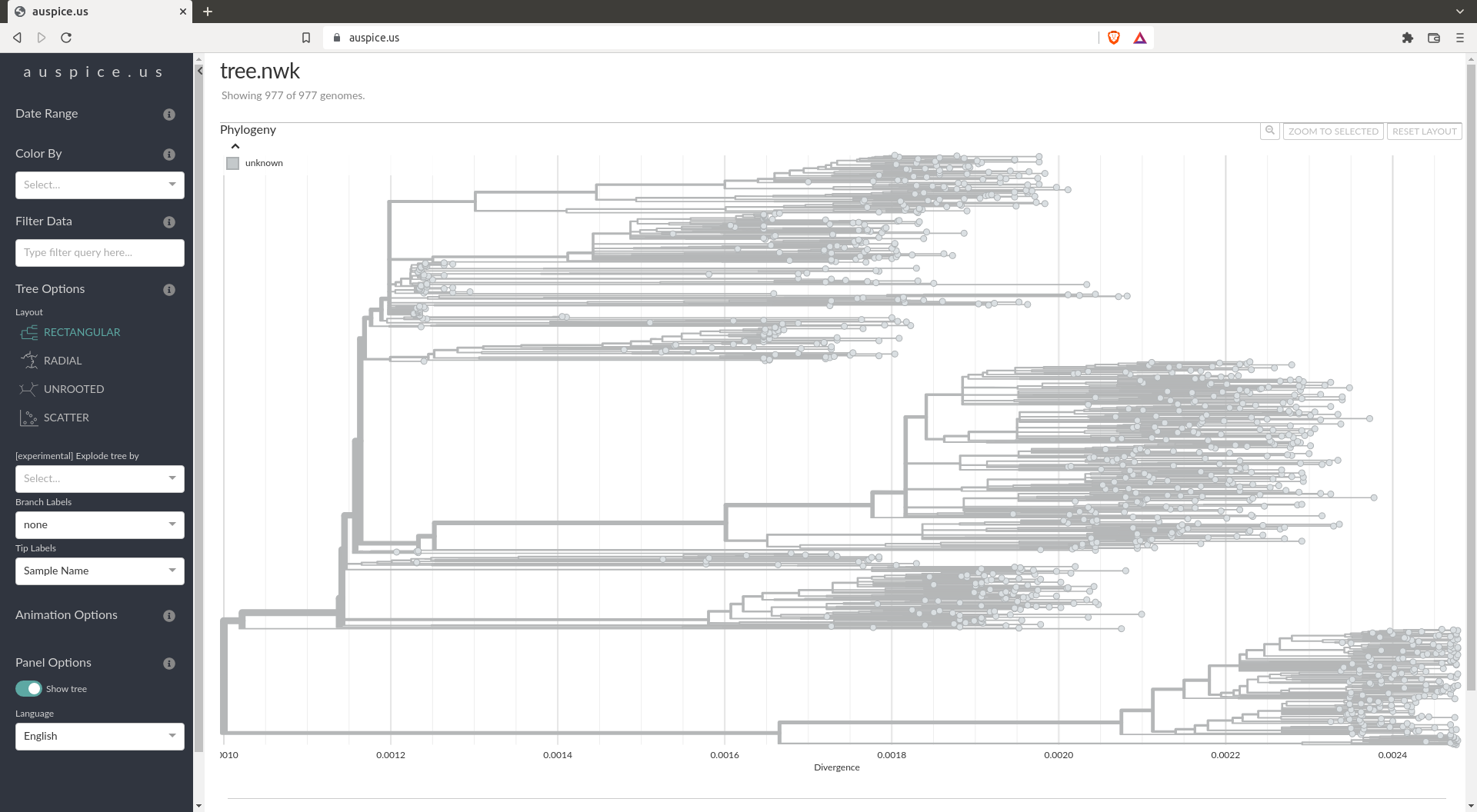
By the looks of the tree computed above, you should notice that it's not usable as it is. For this reason we will refine this tree using the augur refine command. You can once again use something similar to the zika tutorial. Tree refining is usually one of the slowest steps. We again suggest looking at this tree in https://auspice.us/.
The rule:
rule refine:
    message:
        """
        Refining tree {input.tree}
          - estimate timetree
          - use {params.coalescent} coalescent timescale
          - estimate {params.date_inference} node dates
          - filter tips more than {params.clock_filter_iqd} IQDs from clock expectation
        """
    input:
        tree = rules.tree.output.tree,
        alignment = rules.align.output,
        metadata = rules.filter.output.metadata
    output:
        tree = "results/tree.nwk",
        node_data = "results/branch_lengths.json"
    params:
        coalescent = "opt",
        date_inference = "marginal",
        clock_filter_iqd = 4
    shell:
        """
        augur refine \
            --tree {input.tree} \
            --alignment {input.alignment} \
            --metadata {input.metadata} \
            --output-tree {output.tree} \
            --output-node-data {output.node_data} \
            --timetree \
            --coalescent {params.coalescent} \
            --date-confidence \
            --date-inference {params.date_inference} \
            --clock-filter-iqd {params.clock_filter_iqd}
        """
The refined tree should look like:
Ancestral reconstruction and mutations
With the refining of the tree, the main part of the analysis is done. Now we can improve the information we will get when visualizing in Auspice by computing a few additional things. It is usually useful to reconstruct the ancestral state and translate the mutation / compute traits.
This can be done using the augur ancestral augur translate and augur traits commands. It is just like the zika tutorial.
The rules:
rule ancestral:
    message: "Reconstructing ancestral sequences and mutations from {input.tree} and {input.alignment}"
    input:
        tree = rules.refine.output.tree,
        alignment = rules.align.output
    output:
        node_data = "results/nt_muts.json"
    params:
        inference = "joint"
    shell:
        """
        augur ancestral \
            --tree {input.tree} \
            --alignment {input.alignment} \
            --output-node-data {output.node_data} \
            --inference {params.inference}
        """

rule translate:
    message: "Translating amino acid sequences"
    input:
        tree = rules.refine.output.tree,
        node_data = rules.ancestral.output.node_data,
        reference = REFERENCE
    output:
        node_data = "results/aa_muts.json"
    shell:
        """
        augur translate \
            --tree {input.tree} \
            --ancestral-sequences {input.node_data} \
            --reference-sequence {input.reference} \
            --output-node-data {output.node_data}
        """

rule traits:
    message: "Inferring ancestral traits for {params.columns}"
    input:
        tree = rules.refine.output.tree,
        metadata = rules.metadata.output.metadata
    output:
        node_data = "results/traits.json",
    params:
        columns = "country"
    shell:
        """
        augur traits \
            --tree {input.tree} \
            --metadata {input.metadata} \
            --output-node-data {output.node_data} \
            --columns {params.columns} \
        """
Frequencies
Another interesting thing we can add to our analysis is the frequency analysis. This enables you to follow the frequency in time of variants. This is what you can see on the Nextstrain analysis for SARS-COV-2:
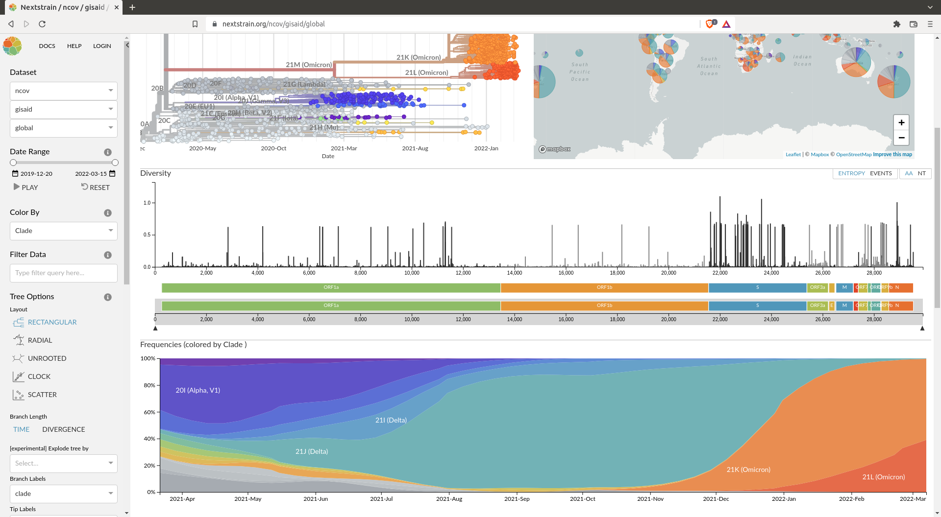
This can be achieved using the augur frequencies command. For this you can inspire yourself from the pipeline used by nextstrain for the SARS-COV-2 builds. To provide the frequencies to Auspice, you can save the tip-frequencies.json directly in you visualisation folder.
The name of this file should be specific for Auspice to detect it. If the output of your augur export (below) is visualisation/NAME.json the name of the frequency file should be visualisation/NAME_tip-frequencies.json
The rule:
rule tip_frequencies:
    message: "Estimating censored KDE frequencies for tips"
    input:
        tree = rules.refine.output.tree,
        metadata = rules.metadata.output.metadata,
    output:
        tip_frequencies_json = "visualisation/SV2_tip-frequencies.json"
    params:
        min_date = "2020-01-01",
        max_date = "2022-03-01",
        pivot_interval = 3,
        pivot_interval_units = "weeks",
        narrow_bandwidth = 0.041,
        proportion_wide = 0.0
    shell:
        """
        augur frequencies \
            --method kde \
            --metadata {input.metadata} \
            --tree {input.tree} \
            --min-date {params.min_date} \
            --max-date {params.max_date} \
            --pivot-interval {params.pivot_interval} \
            --pivot-interval-units {params.pivot_interval_units} \
            --narrow-bandwidth {params.narrow_bandwidth} \
            --proportion-wide {params.proportion_wide} \
            --output {output.tip_frequencies_json} 2>&1 | tee {log}
        """
Visualisation
Now that all the pipeline is built, we need to export the results for visualisation using the augur export command.
You'll also need a small config file for auspice that you should call auspice_config.json. This file should contain the following information:
{
  "title": "Custom build for the Qlife nextstrain workshop",
  "maintainers": [
    {"name": "Your Name"}
  ],
  "panels": [
     "tree",
     "entropy",
     "frequencies"
  ],
  "display_defaults": {
    "map_triplicate": true
  },
  "filters": [
    "country",
    "region",
    "author"
  ]
}
The export rule:
rule export:
    message: "Exporting data files for visualisation auspice"
    input:
        tree = rules.refine.output.tree,
        metadata = rules.metadata.output.metadata,
        branch_lengths = rules.refine.output.node_data,
        traits = rules.traits.output.node_data,
        nt_muts = rules.ancestral.output.node_data,
        aa_muts = rules.translate.output.node_data,
        auspice_config = AUSPICE_CONFIG
    output:
        auspice_json = rules.all.input.auspice_json,
    shell:
        """
        augur export v2 \
            --tree {input.tree} \
            --metadata {input.metadata} \
            --node-data {input.branch_lengths} {input.traits} {input.nt_muts} {input.aa_muts} \
            --auspice-config {input.auspice_config} \
            --output {output.auspice_json}
        """
Combine the whole pipeline in one rule
To combine the whole pipeline in one rule you can create the all rule at the beginning of the snakefile. This rule needs to have as input the visualisation files. The whole pipeline can be run in a simple command snakemake --cores 4.
The rule:
rule all:
    input:
        auspice_json = "visualisation/SV2.json",
        tip_frequencies_json = "visualisation/SV2_tip-frequencies.json"
Results
Visual
You should obtain a visualisation in Auspice that looks like this:
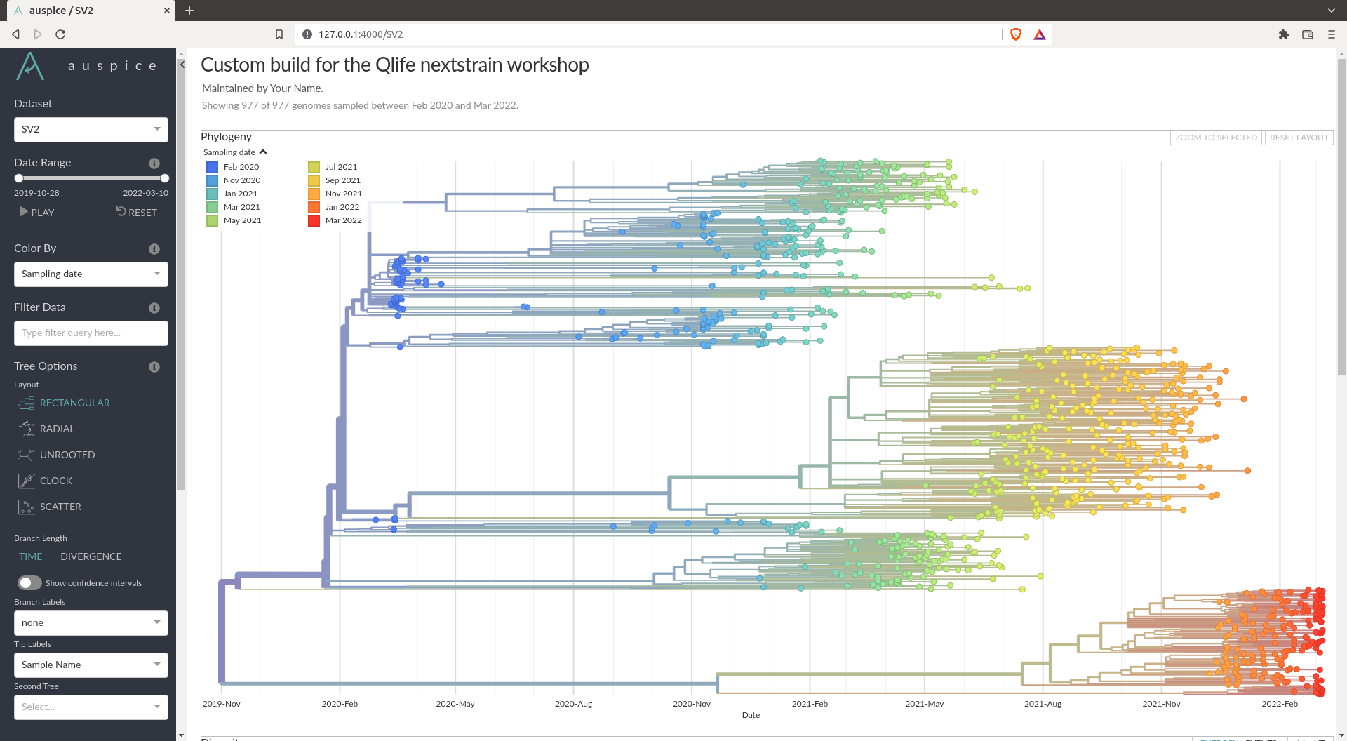
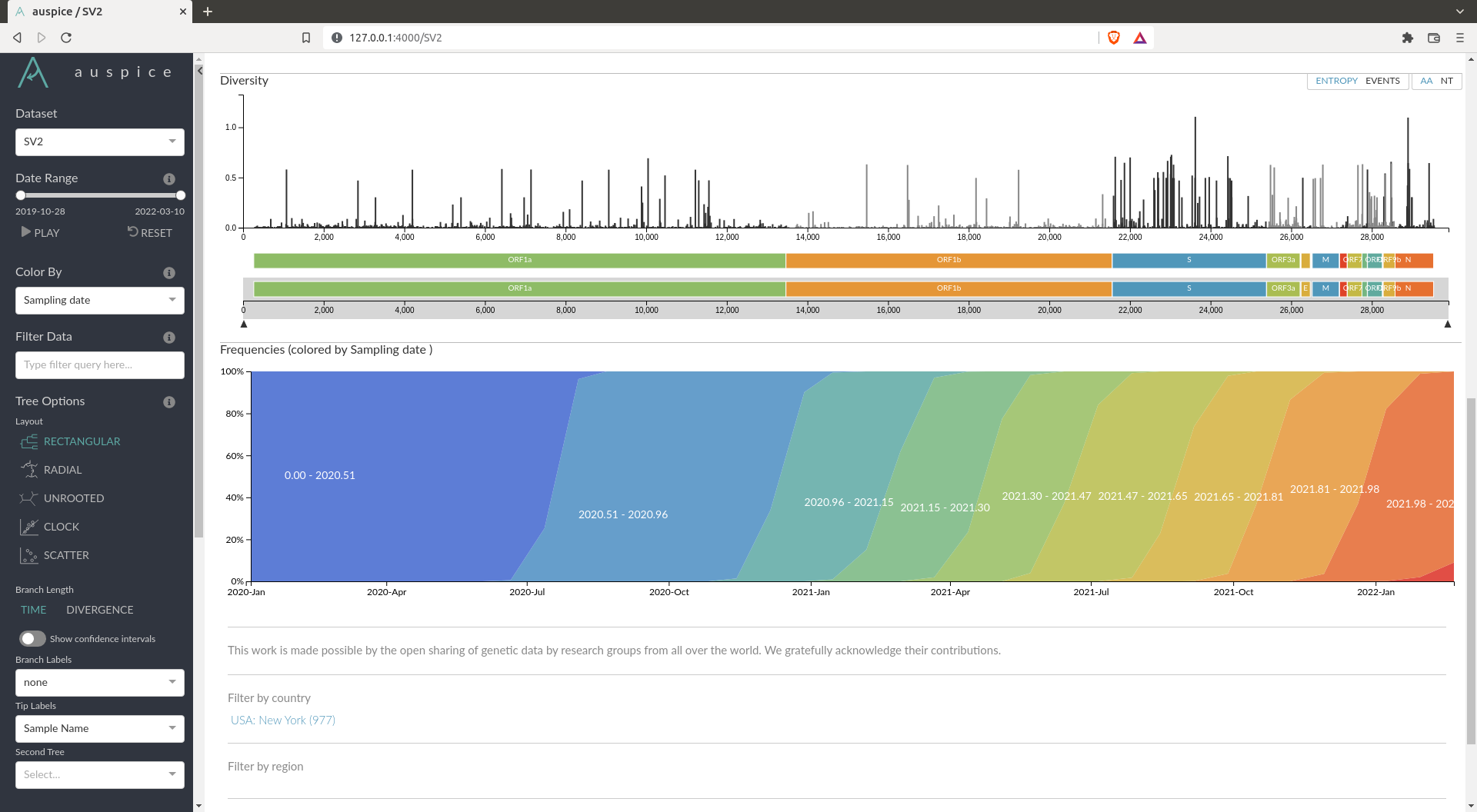 If you obtain something similar to this, you can answer all the questions asked by interacting with this interface.
Answers
How many clades is there in your data ? What do they correspond to ?
In the example given above, you can see there are 3 main clades. These corresponds to the main variants we heard about. The top one are the ancestral variant (alpha, lambda, epsilon etc...), the one in the middle is the Delta wave and the bottom one is the Omicron wave (the most recent).
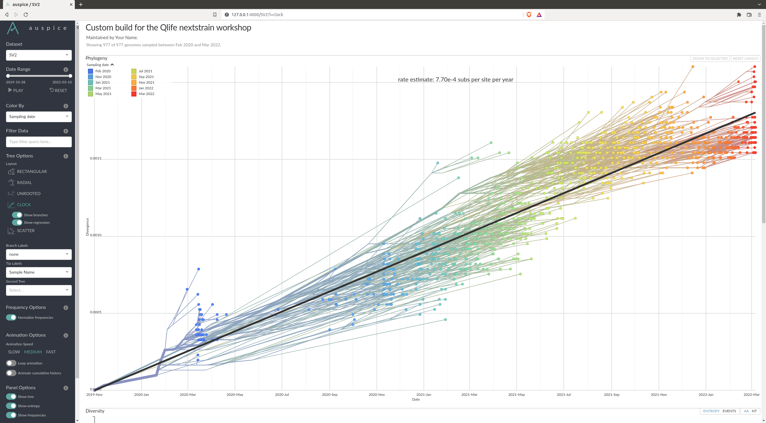
How fast does SARS-COV-2 evolve overall ?
My looking at the clock plot in Auspice, we see in my example that we find a mutation rate of $7.7\cdot 10^{-4}$ substitutions per site per year.
Is the root of the tree correctly inferred ?
In my example it seems the root of the tree is not correctly inferred. The root of the tree is placed between the omicron and delta variant. From the current knowledge we have, it seems the ancestral variants should be closer to the root, while the Delta and Omicron variants came later.
Where are most of the mutations happening ? What does this gene correspond to ?
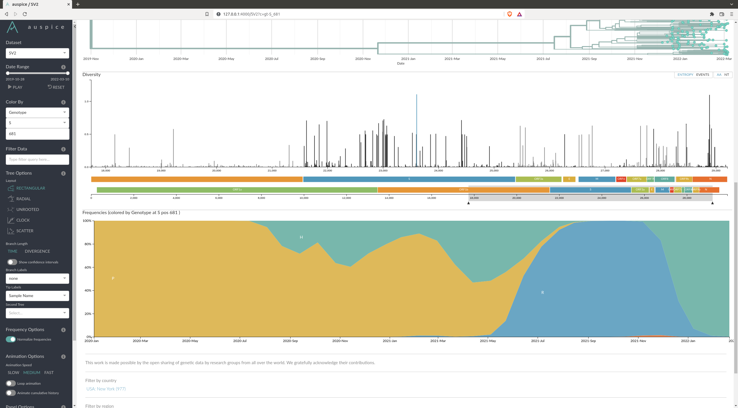
By looking at the diversity plot one can see that most of the mutations happen in the S gene. This gene is the spike protein that is on the outside of the virus. It is usually what is targeted by the immune system via antibodies. Hence it is probably under higher selection pressure, which means mutations accumulate faster than elsewhere.
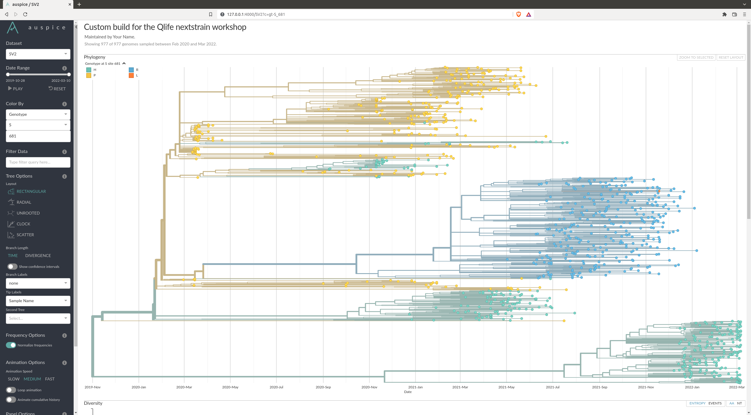
What are some of the mutations characterizing the different variants ?
There are many mutations that differ from variant to variant. An example of one can be the position 681 of the spike protein (S681), where you can see a clear distinction between the variants.
You can check some other that are documented here: https://covariants.org/shared-mutations